Fixing Faults

Kasey W. Schultz

kwschultz@ucdavis.edu
github.com/kwschultz
Advisor: Prof. John Rundle

How do you completely re-index a fault model? Creative problem solving example.

I have recently found that the UCERF3 fault model we use for our Virtual Quake simulations of the California fault system has some faults that are slipping the wrong way. For example, one of the biggest problems in the model is that the northern half of the San Andreas fault slipping one way and the southern half of the fault slipping the opposite direction; in clear contrast to reality. After inspecting the model further, I suspect that a large number (>25%) of the 313 faults in the UCERF3 model are slipping in the wrong direction. This presents a major problem for earthquake simulators, where the reversing the slip direction of a fault will reverse the stress interaction on nearby faults (e.g. changing a stress increase to a stress decrease).
In addition to enforcing faults to slip in the proper direction, we want to re-index the entire fault model in a more convenient manner for our own data analysis. For easy iteration over the fault model data structure we would like the fault sections and elements to be indexed in their physical order of appearance along the fault.

How can we fix faults that are slipping the wrong direction?
We can build tools to detect problematic faults and to re-align them properly.

In this post I will describe the methods and tools I have developed (with important contributions from fellow graduate student John Wilson) to fix the UCERF3 fault model. I will also include links and explanations along the way of the python scripts I wrote that allow us to further improve the model each time we find a new instance of a fault slipping the wrong direction. Additionally, the scripts will re-index the entire fault model such that all indices (of sections and elements) appear in the correct order along each fault. We need to apply the following fixes:

Group single faults that come labeled as multiple faults (e.g. San Andreas is labeled as more than 10 different faults)
Re-index the fault model so that the indices (of sections and elements) appear in order along the direction of the fault
Assert that the faults actually slip in the correct direction

These scripts are fault_match.py, sectioning.py, elements.py and vertices.py; all are found in my github repository github.com/kwschultz/VQModels/. These tools utilize regular expressions, the Python geospatial library Shapely, the Python module quakelib that we develop and provide along with Virtual Quake, and good old-fashioned re-indexing math.

Overview of the fault model data hierarchy

Lets take a brief moment to discuss the hierarchy of finite fault models. A fault model is essentially a small database-like file of fault properties with multiple indices. Each level of the data is bulleted below, and as an example the Elsinore fault is shown in the annotated Google Earth image below.

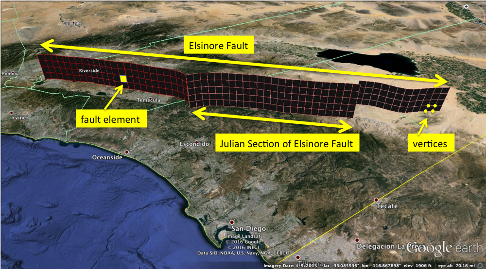
A fault is a planar surface on which dislocations occur; earthquakes. A fault's physical properties can vary as one moves along the fault, but the properties do not very that much. The first index of our fault model is the fault ID . All other data structures belong to one and only one fault.
A fault section is the next level of data structure. Each fault has multiple sections, and the fault's physical properties are constant within a section. This is the second index for our fault model, every section has a unique section ID. Each section belongs to one and only one fault.
A fault element is the interacting member of the physics-based simulation. Every fault is comprised of fault elements, and for the UCERF3 model, we discretize the faults into 3km by 3km square elements. Our stress interaction physics is used to determine to stress increases and decreases between each pair of fault elements in the model due to stress loading and earthquakes. An earthquake is an event where groups of fault elements slip. Fault elements represent the third index for our fault model. Every element has a unique element ID, and each element belongs one and only one section.
A vertex is a point in latitude/longitude/depth space that defines one corner of a square fault element. This is the fourth index for our fault model. Every fault element has four vertices (lets call them vertex_0, vertex_1, vertex_2, vertex_3), and each vertex has a unique vertex ID. The order of the vertices for a particular fault element matters. The vector from vertex_0 to vertex_2 sets the slip direction for the fault element. Therefore, if we switch the order of the vertices within an element, we are switching the element's slip direction.

How do we know if a fault is slipping the wrong direction?

First, what is the direction of a fault? In geological terms, each fault is given a slip direction by specifying its strike angle (and also a rake angle but its not important here). The strike angle is measured clockwise from north as shown in the figure below for the Elsinore fault in southern California.

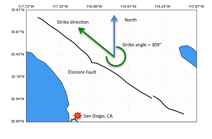
The problem with faults in the UCERF3 model slipping the wrong way is due to an improperly prescribed strike angle. And after an exhaustive inspection of the model, faults either have the correct strike angle or they are 180 degrees off. The Elsinore fault as shown has the correct strike angle in the UCERF3 model. However, the strike angle for the northern half of the San Andreas fault is around 130 degrees, while the strike angle for the southern half is around 300 degrees. Meaning that the northern half slips northward while the southern half slips southward, a clear error.

The method I have developed for re-aligning the faults in the correct direction uses a dictionary of target strike values that we want the faults to have and then iterates through all levels of the fault model data structure and aligns the indices to appear in order along strike. This method cannot properly fix the entire fault model off the bat, since we do not have easy access to a database of the correct strike values. The first iteration of these fixes has involved checking the USGS's own fault database and recording the correct strikes by hand for 15 major faults (listed here). However, this method can be used to improve the model as readily as new, accurate strike data can be ingested. The best approach would be a web-scraping approach to grab the correct strike data from the database, however in initially exploring this option I have found a big complication; there is no guaranteed database entry for each UCERF3 fault name.

Lets re-group the faults

The UCERF3 model treats the sections of many major faults as their own faults. For Virtual Quake, the distinction between faults and fault sections has an impact on the simulation. I have developed another algorithm in the simulation that uses a fault's geometry information (total area, length, etc.) to determine the stress drops for that fault. The stress drops are used in the simulation to determine how much each fault element should slip during an earthquake given the levels of stress. Since the UCERF3 model as provided to us is over-faulted, we must combine the given faults into the smaller number of real faults that we have in California.
For example the Coachella, Cholame, and Big Bend sections of the San Andreas in southern California all have different fault IDs and belong to different "faults". Lets look at the section names and fault IDs for these San Andreas sections.

San_Andreas_Coachella_rev_Subsection_0 with fault ID 295
San_Andreas_Coachella_rev_Subsection_1 with fault ID 295
...
San_Andreas_Cholame_rev_Subsection_0 with fault ID 285
San_Andreas_Cholame_rev_Subsection_1 with fault ID 285
...
San_Andreas_Big_Bend_Subsection_0 with fault ID 287
San_Andreas_Big_Bend_Subsection_1 with fault ID 287
...

Just inspecting the names of these sections tells you that they all belong to the San Andreas fault. And there we have it, we only need to look at the names of each fault section to determine which fault to match the section to. All we need to do is to use regular expressions to trim off the non-fault-specific bits of each section name and that trimmed section name will be the unique fault name. This is exactly the word slicing and dicing that fault_match.py does, trimming off non-unique fault identifiers in the section names like "_Subsection_0", "_rev", "_North", etc. After parsing the section names, we have a list of the unique fault names. Then we just need to keep a single fault ID for each unique fault name and assign that fault ID to each section that matches the unique fault name. This reduces the 313 faults in the original UCERF3 model to 256 unique faults.

We need the sections to appear in order along the fault strike

The sections provided in UCERF3 come organized in alphabetical order by section name, not in their actual order along the fault. There are multiple reasons why we want the section IDs and hence the sections to appear in order of appearance along the strike of the fault. This re-indexing will be more difficult than name matching because the section data only contains a name, an ID, and a list of elements that belong to that section.
In order to align the sections along the fault strike, I must use the positional information of the fault elements within each section. Then using say, a mean position of the elements within each section along with the target fault strike I can re-assign section IDs within a fault. If I can compute the distance along the fault of each section, then I have computed a score with which I can rank the sections in order along strike and re-assign the section IDs. This is where Python's Shapely module comes in handy.
After computing the mean location (x,y) for each section within a fault, I need to create a Shapely Line object that has endpoints at each end of my fault. To do this I just select the pair of sections that have the farthest separated mean locations. However, there is a degeneracy here and this fault line I am creating needs to point in the direction of the correct strike. To do this I created functions that compute the strike angle of the line segment and choose the direction of the line to minimize the difference between the computed strike and the target strike for this fault - being careful here when computing the difference between angles. For example, what is the angular difference between a strike of 359 degrees and 1 degree? It's not 358 degrees.
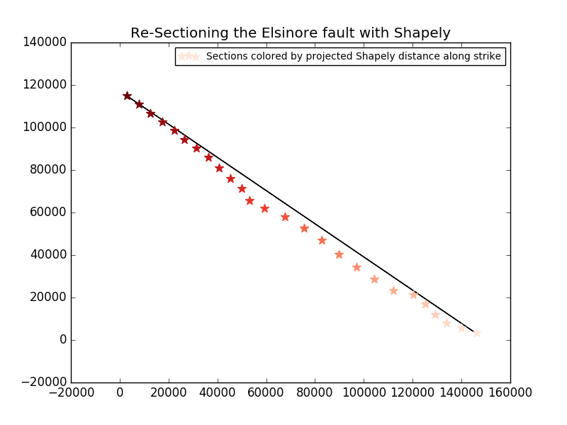
Once I have created the Shapely line object that is in the correct strike direction, I can use Shapley's project() function to compute the distance of each section's mean location along the fault strike from 0 to 1. I then use these scores and re-assign section IDs within the fault to appear in order along strike. An example is shown in the figure below. The color of the stars indicate the section's projected distance along strike (darker is farther) and the black line in the fault-strike-aligned Shapely Line object. All of this is done by sectioning.py.

We also need the elements to appear in order along the fault strike

Since the sections provided in UCERF3 come organized in alphabetical order by section name, this produces discontinuities in element IDs when stepping along a fault in the strike direction. Also the strike is not continuous within a fault, and can flip 180 degrees from section to section within a fault. Furthermore, since the element numbering increases "down" each fault with increasing depth, we cannot simply detect an incorrect element ordering and reverse it since the reversed ordering would increase "up" the fault with decreasing depth. The figure below illustrates a typical case of problematic element ordering and the corrected version.

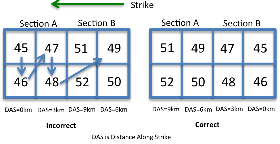
If we cannot reverse the element ordering, what can we do? In order to change the element numbering along strike while preserving the element ordering convention (also used by Virtual Quake) of increasing element IDs with depth, we can just reorder each column of elements. We can use the provided, though incorrect, variable called "distance along strike" (or "DAS") that is specified for every vertex and hence every element. Even though we know the elements are out of order and hence the distance along strike values are out of order, they are still constant with respect to each column as shown in the figure above.
As such I use the prescribed DAS values as the index for each column of elements and build a dictionary of all element IDs in each DAS column. I then compute the strike angle of the line segment connecting the minimum and maximum element ID in each section and determine if the elements are reversed by comparing this to the correct strike angle. If the section has elements out of order, I iterate over the dictionary of elements indexed by DAS and reverse the order of the columns of elements in the section. It is then straightforward to use the DAS index, the number of elements per column (observed to be constant within sections) and the minimum element ID in each section to re-index the element IDs within the section. Then one final iteration the new element IDs in order to set the correct DAS values for each element's vertices, utilizing the lengths of the elements computed from vertex locations.
All of this is done by elements.py, which finds that 1076 of the 2606 (41.3%) UCERF3 fault sections have elements indexed in the opposite order of the strike direction.

Last and most importantly, the vertex ordering within the elements must align with the strike

During a Virtual Quake simulation, we compute the slip direction for a fault element using the vector between its first and third vertex (the ones at the top of the square). This slip direction goes into Greens function matrix calculations which set the stress interactions for the simulation. If the vertex ordering does not match the true strike direction for the fault, the fault elements will slip in the wrong direction and we will not properly model stress interactions.
Because we are now operating at the lowest level in our fault model data structure, this index remapping is the simplest. We only need to iterate over the fault elements once and check that the strike computed from the vertex ordering matches the true strikes for the faults. If they do not match, simply switch the ordering of the vertices within the fault element. All of this is done by vertices.py, which finds that 1561 of the 21833 (7.2%) UCERF3 fault elements have vertices indexed in the opposite order of the strike direction. This number will only increase as more accurate strike data can be ingested.

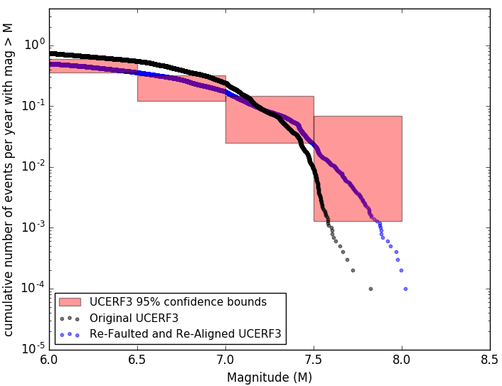
The effect of re-faulting and re-aligning on simulated earthquakes

After applying the four python scripts to the UCERF3 fault model, I reduce the number of faults from 313 to 256 and reverse the slip direction on 7.2% of the 21833 fault elements (correcting the slip direction for 15 major faults). The fault grouping operation gives us fewer faults with larger surface areas, which allows Virtual Quake to prescribe more displacement given the same stress accumulation per earthquake. These two effects have a noticeable effect on simulated earthquake rates. The plot below shows two 10,000 year simulations of the UCERF3 model before and after fault regrouping and slip realignment. The vertical axis is the number of earthquakes, the horizontal axis is the magnitude. The red boxes are the 95% confidence bounds for the observed earthquake rates in California from 1932 to 2011; hitting more boxes is better. The vertical axis is on a logarithmic scale, so being able to distinguish the two curves means there is a very large difference in the number of earthquakes of a given magnitude. Further improvements to the fault model will make this difference even more apparent, and give us a more physically accurate fault model.